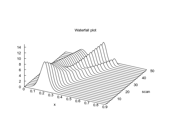
# Waterfall plot created using plot style "splot with filledcurves"
#
# Note that scan lines must be plotted from back to front
# in order for the depth-occlusion visual effect to work.
#

# Generate data
Gauss(x,mu,sigma) = 1./(sigma*sqrt(2*pi)) * exp( -(x-mu)**2 / (2*sigma**2) )
A(x) = Gauss(x, 0.2, 0.05)
B(x) = 0.8 * Gauss(x, 0.2 + s, 0.03)
C(x) = 0.1 * Gauss(x, 0.2 + 1.5*s, 0.02)

set xrange [0.0:1.0]
set sample 101

set table $DATA
s = 0.0
do for [j=1:50] {
    f = (75-j)/75.
    F(x) = f * A(x) + (1-f) * B(x) + C(x)
    plot F(x)
    s = s + 0.005
}
unset table

# set print "DATA"
# print $DATA

set title "Waterfall plot"   offset 0,-5
unset key
set view 42, 27, 1, 1.2
set xyplane at 0
set xtics scale 0
set ytics scale 0 10,10,50
set xrange [0:0.9]
set yrange [0:50]
set zrange [ 0.0 : 15.0 ]
set xlabel 'x'
set ylabel 'scan'

splot for [scan=48:2:-2] $DATA index scan \
      using 1:(scan):2 with filledcurves lc "black" fc background


Click here for minimal script to generate this plot
